
You need to know some maths for A level Biology. This includes knowing how to interpret averages (mean, median and mode), ranges, and standard deviations to work out whether an experiment can be said to have shown an effect or not. Master this early on and it will not help you with exam questions, but also make it easier for you to learn the bits of the course that are explained using these statistical methods.

Why does Biology need so much data?

Maybe the guy at the back is just big for his age?
Researchers often want to compare two or more things. Which species of frog is heavier? Which type of soil grows taller plants? At what temperature do these bacteria divide fastest? At which pH are fish most active?
The biological world is complicated, so multiple, repeated measurements are usually required.
There are three main reasons for taking multiple measurements:
Measurement errors. It’s hard to take measurements in the real world. Even if you re-measure the exact same thing, and even if you use a well-calibrated tool, you might get a slightly different result each time. Maybe you can’t hold the tool still enough, or you can’t read it clearly, or the thing you’re measuring moves. These are precision errors.
Individual variation. If you want to ask a general question about a whole population, eg “do robins sing more than blackbirds” then you need to measure data from more than two individuals. If you only use two, you might randomly pick outliers; maybe you get a particularly perky robin, or a lazy/sick blackbird. Similarly, if you sample a small area of a larger region, you may not pick a representative area.
Uncontrolled variables.There will nearly always be variable-influencing factors that you’re not aware of, or unable to control. Maybe there are changing sounds or smells in the environment, subtle changes in light, or in the birds’ blood-sugar levels. These can affect individual measurements in unpredictable ways.
All of these things can affect the value you record, making any one single measurement unreliable. So researchers normally end up collecting large sets of measurements. In this way they can get a much better idea of what’s really going on.
Why does Biology need Statistical techniques?
Plotting lots of repeated measurements for different datasets on the same graph can create a confusing mess. Also, “the data look different to me” isn’t good enough for science.
Reducing each dataset to just two or three values makes it much easier to compare. In fact, it’s so simple that such data can be understood even without a graph, so values are often presented very simply in a table.
Calculating Averages in Biology
There are three types of average: mean, median, and mode. They all reduce the data set to one single number.
This is useful for comparisons. For example, if you let a frog jump ten times, measuring the length of every jump, you can calculate their average jump length. You can then compare that single number to the average jump length from another frog to find out which jumps further.
Calculating the Mean
The most important type of average for A level Biology is the mean. It’s also what most people are talking about when they say “average” in everyday life.
To find the mean, add up all the numbers, then divide by how many numbers there were. You end up with just one number.
Here’s an example dataset:
| Set 1 | 3 | 4 | 5 | 5 | 5 | 6 | 6 | 6 | 7 | 8 | total = 55 / n = 10 / mean = 5.5 |
| Set 1 | 3 | 4 | 5 | 5 | 5 | 6 | 6 | 6 | 7 | 48 | total = 95 / n = 10 / mean = 9.5 |
| Set 1 | 3 | 4 | 5 | 5 | 5 | 6 | 6 | 6 | 7 | 48 | central number(s) = 5 and 6 / median = 5.5 |
| Set 1 | 1 | 3 | 5 | 5 | 5 | 5 | 6 | 6 | 7 | 48 | mode = 5 |
| Set 1 | 50 | 50 | 50 | 50 | 50 | 50 | 50 | 50 | 50 | 50 | mean = 50 / median = 50 / mode = 50 | ||
| Set 2 | 25 | 30 | 35 | 40 | 50 | 50 | 60 | 65 | 70 | 75 | mean = 50 / median = 50 / mode = 50 | ||
| Set 3 | 1 | 2 | 3 | 4 | 50 | 50 | 96 | 97 | 98 | 99 | mean = 50 / median = 50 / mode = 50 |
The averages are the same! By themselves, averages only tell you one small part of the story.
What is Range / why is it useful
One of the big differences betwen the datasets above is the range of numbers that appear.
The range is the range-of-values that appear, from the lowest to the highest.
| Set 1 | 50 | 50 | 50 | 50 | 50 | 50 | 50 | 50 | 50 | 50 | lowest value = 50 / highest value = 50 / range = 50 to 50 | ||
| Set 2 | 25 | 30 | 35 | 40 | 45 | 55 | 60 | 65 | 70 | 75 | lowest value = 25 / highest value = 75 / range = 25 to 75 | ||
| Set 3 | 1 | 2 | 3 | 4 | 50 | 50 | 96 | 97 | 98 | 99 | lowest value = 1 / highest value = 99 / range = 1 to 99 |
Set 1 has a range of 50 to 50. So you can reasonably predict that the next measurement would likely be 50 too
Set 2 and Set 3 have wider ranges. There are a wider range of possible values that might be measured, so it’s harder to predict what the next measurement might be.
A wide range might indicate that your measurement technique is very unprecise, or that there is a wide natural variation in the thing you are measuring, or that there is another factor affecting your measurements.
But a wide range might also just mean there were one and two weird outliers in the data. So you need to be careful when using this value. Here is a set with one odd measurement, which might be due to a measurement error.
| Set 4 | 50 | 50 | 50 | 50 | 50 | 50 | 50 | 50 | 50 | 90 | lowest value = 50 / highest value = 90 / range = 50 to 90 |
| Set 1 | 25 | 42 | 48 | 50 | 50 | 50 | 50 | 52 | 58 | 75 | values clustered around mean = low standard deviation | ||
| Set 2 | 25 | 30 | 35 | 40 | 45 | 55 | 60 | 65 | 70 | 75 | values spread out away from mean = high standard deviation |
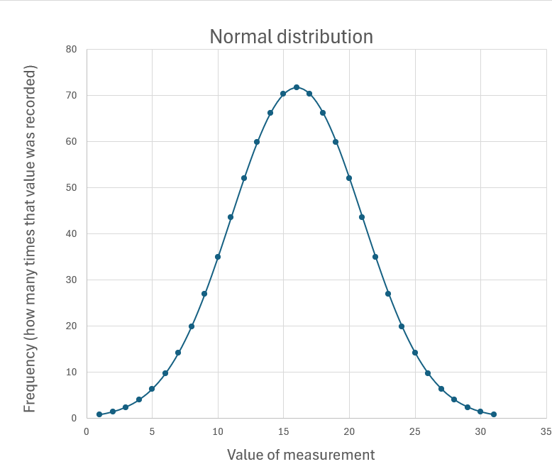
To understand Standard Deviation, think about a situation where you have made very many measurements, so that you have multiple measurements at each possible value. Now plot these on a graph (see below). In biology, you usually see that the graph forms a bell shape. This is called a “Normal distribution”.
Normal distributions are symmetrical, so the mean, mode, and median are all the same, appearing at the centre of the graph (mean, median, and mode = 16 in this example). In normal distributions, most measurements are near the average, so there is a peak in the middle of the graph.
(Sometimes, you’ll find a curve is skewed a bit to one side. This separates out the mode, median and mean values. But for our purposes, I’m going to stick to thinking about the symmetrical graph.)
How wide the curve is matters a lot, because it affects how much two sets of data overlap. Compare these two examples below. Both have one set of data where the mean is 14 (plotted in orange), and another set where the mean is 20 (plotted in blue).
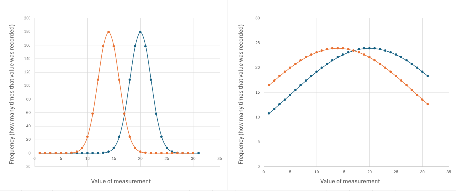
There is the same amount of data in both graphs, and the averages haven’t changed. But there is a lot less overlap between the two datasets in the example to the left. The data on the right is a lot more spread out away from the average values.
When datasets overlap a lot, you need to be very careful that you definitely have enough data to be sure their means really are different. If you have a small data set with a lot of variation, then adding extra measurements can make a big difference to the mean.
What is Standard Deviation
Standard Deviation tells you how widely the data is spread out in a normal distribution. Its symbol is sigma, “σ”.
You’re very unlikely to be asked to calculate standard deviation in an exam, and it takes a while to explain so I’m not going to go through it here (don’t worry they’d give you the equation if you did have to do this).
But you do need to know what it tells you.
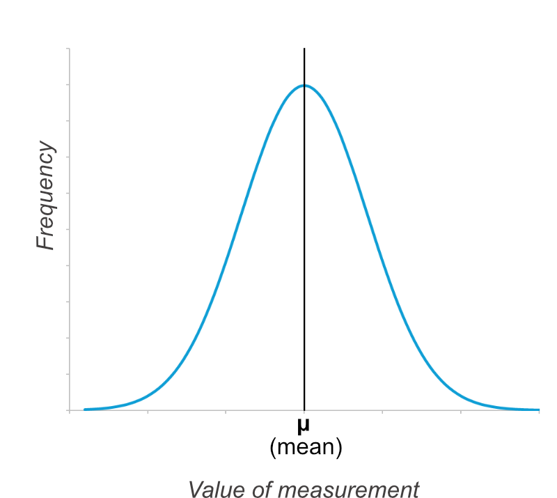
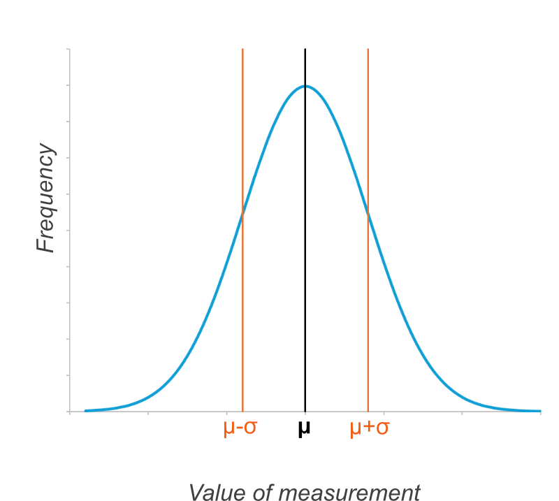
Here is the basic normal distribution graph again. The graph is symmetrical and the mean (μ) is in the centre.
Now here is the same graph, but two more values are marked on the x-axis, shown by orange lines. These are the value of the mean minus one standard deviation (μ-σ), and the value of the mean plus one standard deviation (μ+σ).
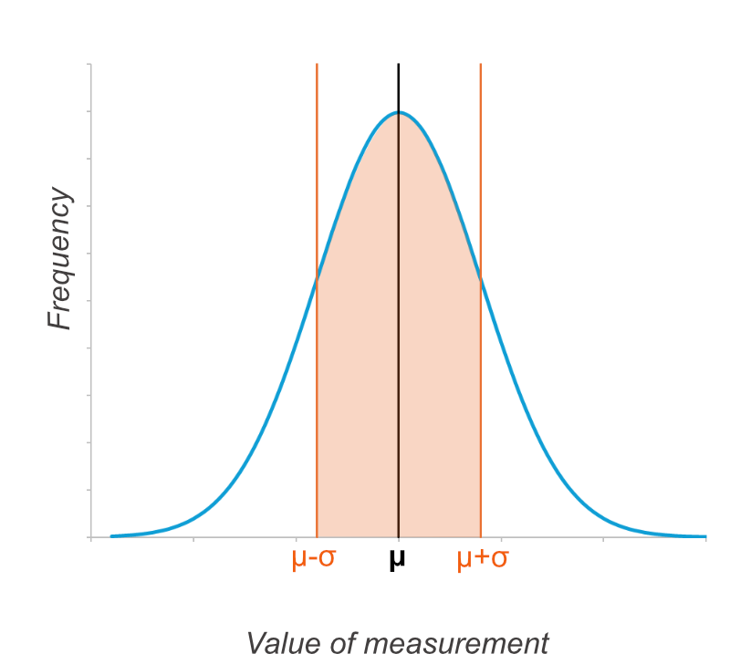
If you colour in the bit of the graph that is within one standard deviation of the mean (from μ-σ to μ+σ), then on any normal distribution, 68.27% of the data points will lie within this area. You don’t need to remember that percentage, but remember it is always the same.
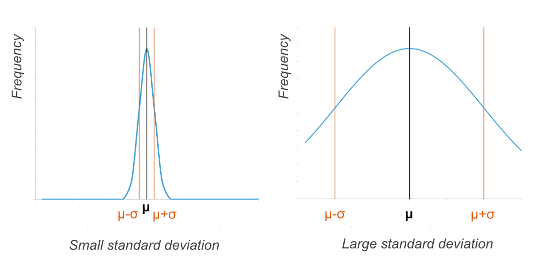
This means that if the standard deviation is a small number, you know most of the data points are close to the mean. This gives you more confidence that the mean is a useful value for comparison.
The graphs below have the same X-axis. Both are normal distributions with the same mean. But the one on the left has a small standard deviation, and the one on the right has a high standard deviation. (Some of the data from the right-hand graph falls outside the values shown on the graph.)
How to tell if there is a significant difference between values using the mean and standard deviation
!! Ok so this is the important bit we’ve been building up to !!
In a normal distribution, most of the data (68.27%) falls within one standard deviation of the mean. This is the area between μ-σ and μ+σ.
To work out whether it’s just chance that the means are different, or whether it’s a real effect, you need to check whether this area overlaps bewteen the two sets of data.
If the areas between μ-σ and μ+σ overlap, the difference is not considered significant.
There are different ways of presenting the data.
Standard Deviations Using Numbers - example
An example:
Set 1: mean (μ) = 50, standard deviation (σ) = 8
Set 2: mean (μ) = 40, standard deviation (σ) = 3
Are these sets of data significantly different? Look at the areas between μ-σ and μ+σ
Set 1: μ-σ = 42 and μ+σ = 58
Set 2: μ-σ = 37 and μ+σ = 43
Do these areas overlap? Yes they do (both include 42-43). So you can not consider the two data sets significantly different.
(Also worth knowing: nearly all the data (95.45%) falls within two standard deviations (between μ-2σ and μ+2σ) - so if these two areas don’t overlap you can be even more sure the two sets of data really are different.)
Standard Deviations Plotted on Graphs - example
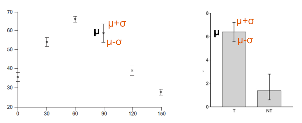
On graphs, the mean is plotted as usual, with a dot or column. Extra lines extend out to show the area from μ-σ to μ+σ. This can make it more obvious whether areas overlap or not (unless they are super close in which case numbers are more useful).
Standard Deviation Exam Past Papers
Example Exam Question 5
Question 5 answers found at the bottom of this web page
Understanding Standard Deviations from Graphs
Example Exam Question 6
Question 6 answers found at the bottom of this web page
Example Exam Question 7
Question 7 answers found at the bottom of this web page
Graphs and Tables in A level Biology
If you’re not confident with questions that include graphs and tables, see the recent blog post “How to Approach A level Biology Graph and Table Questions: Tips and Exam Question Pack”, which offers more useful tips for navigating them during exams, and more exam questions to practice with.
Answers to example exam questions
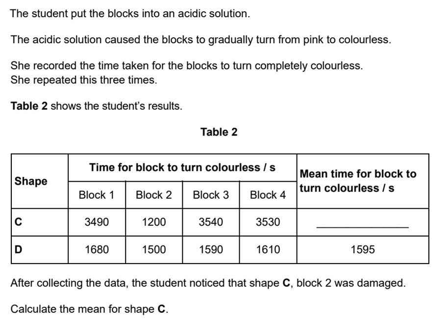
The data for the damaged block should be ignored. The mean for shape C is 3520 seconds
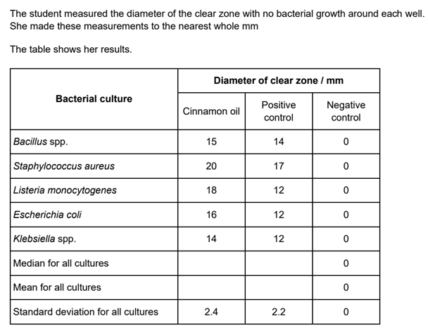
Cinnamon Oil median = 16, mean = 17 ….. and ….. Postive Control median = 12, median = 13
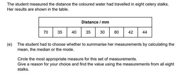
Median = 41. This avoids the outliers affecting the value as would happen if you used the mean. And the sample size is too small to use the mode (there are no repeated values)
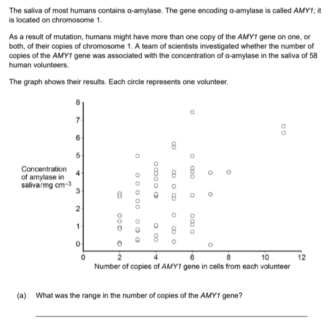
The range is 2 to 11
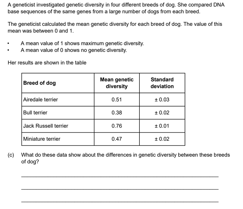
Bull terrier genetic diversity is significantly the smallest of the breeds shown, meaning it the most inbred. Jack Russell genetic diversity is significantly the greatest. The genetic diversity of Miniature terrier and Airedale terriers are similar with no significant difference between the two.
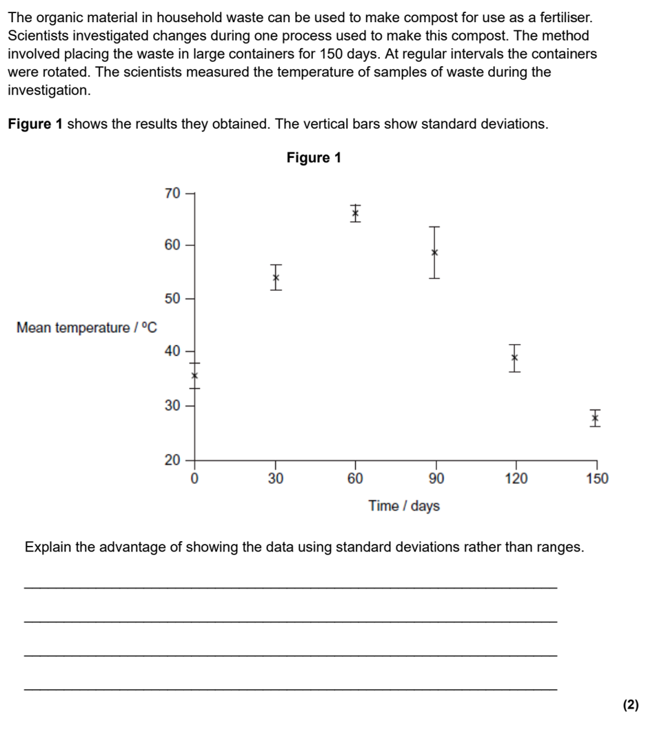
Standard deviation is spread of data around the mean; using standard deviation reduces effect of anomalies/ outliers; standard deviationcan be used to determine if (the difference in results is) significant/not significant/due to chance /not due to chance
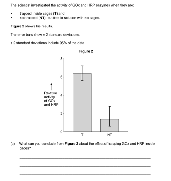
Trapping increases enzyme/GOx/HRP activity; the difference/increase is significant (it is unlikely to be due to chance as the standard deviations do not overlap)